Impact of Urbanization on Biodiversity

This project analyzes changes in the Biodiversity Intactness Index (BII) in Phoenix, Arizona (Maricopa County) between 2017 and 2020. The analysis aims to understand the impact of urban expansion on local biodiversity, as Phoenix has experienced significant urban development in recent decades.

Link to github repo

Course Website: EDS 220

About

Purpose: This project analyzes changes in the Biodiversity Intactness Index (BII) in Phoenix, Arizona (Maricopa County) between 2017 and 2020. The analysis aims to understand the impact of urban expansion on local biodiversity, as Phoenix has experienced significant urban development in recent decades.

Highlights:

• Data Exploration: Accessing and extracting geospatial data through the pystac_client API,focusing on specific collections and spatial extents. Implementing raster data processing using rioxarray.

• Temporal BII Analysis: Analyzing changes in the Biodiversity Intactness Index (BII) across Phoenix from 2017 to 2020, with particular emphasis on areas maintaining high biodiversity values (BII ≥ 0.75). Quantifying percentage changes to measure the impact of urban development on local ecosystems.

• Spatial Visualization: Developing comprehensive visualizations using multiple data layers to illustrate biodiversity changes. Combining vector and raster datasets to create informative maps that highlight areas of significant BII loss.

About the data:

This study utilizes two primary datasets to analyze biodiversity changes in Phoenix. The Biodiversity Intactness Index (BII) data is sourced from Microsoft Planetary Computer’s STAC catalog’s io-biodiversity collection, specifically focusing on temporal changes between 2017 and 2020. The analysis area is defined by a bounding box with coordinates [-112.826843, 32.974108, -111.184387, 33.863574] encompassing the Phoenix metropolitan region. The study area boundaries are defined using the Phoenix subdivision shapefile, obtained from the 2020 TIGER/Line® Shapefiles published by the US Census Bureau, which provides detailed county subdivision boundaries for Arizona.

Source:

Microsoft Open Source, Matt McFarland, Rob Emanuele, Dan Morris, & Tom Augspurger. (2022). microsoft/PlanetaryComputer: October 2022 (2022.10.28). Zenodo. https://doi.org/10.5281/zenodo.7261897 Accessed: 2024-12-02

2020 TIGER/Line Shapefiles (machinereadable data files) / prepared by the U.S. Census Bureau, 2020 https://www.census.gov/cgi-bin/geo/shapefiles/index.php?year=2020&layergroup=County+Subdivisions Accessed: 2024-12-02

Set Up

We will use the following libraries and set-up through this analysis

# Import libraries
import os
import pandas as pd
import numpy as np
import matplotlib.pyplot as plt # To plot the final figure
import matplotlib.pyplot as mlines # To add legend to final figure
import geopandas as gpd # To work with shapefiles
import rioxarray as rioxr # To work with rasters
import contextily as ctx # To add a basemap

from pystac_client import Client # To access STAC catalogs

import planetary_computer # To sign items from the MPC STAC catalog

from IPython.display import Image # To nicely display images

# Set option to display all columns
pd.set_option('display.max_columns', None)

Data Exploration

1. Before retriveing any data, update .gitignore with the entire data directory for best version control efficiency.

2. Download and import TIGER county subdivisons shapefile for Arizona in 2020.

3. Add a base map from the contextily package

# Load boundary data
arizona = gpd.read_file(os.path.join('./data/','tl_2020_04_cousub.shp'))
arizona.head()

# Filter for Phoenix
phoenix = arizona[arizona['NAME'] == 'Phoenix'] 
phoenix.head()

# Get general information about data
phoenix.plot()
phoenix.crs

<Geographic 2D CRS: EPSG:4269>
Name: NAD83
Axis Info [ellipsoidal]:
- Lat[north]: Geodetic latitude (degree)
- Lon[east]: Geodetic longitude (degree)
Area of Use:
- name: North America - onshore and offshore: Canada - Alberta; British Columbia; Manitoba; New Brunswick; Newfoundland and Labrador; Northwest Territories; Nova Scotia; Nunavut; Ontario; Prince Edward Island; Quebec; Saskatchewan; Yukon. Puerto Rico. United States (USA) - Alabama; Alaska; Arizona; Arkansas; California; Colorado; Connecticut; Delaware; Florida; Georgia; Hawaii; Idaho; Illinois; Indiana; Iowa; Kansas; Kentucky; Louisiana; Maine; Maryland; Massachusetts; Michigan; Minnesota; Mississippi; Missouri; Montana; Nebraska; Nevada; New Hampshire; New Jersey; New Mexico; New York; North Carolina; North Dakota; Ohio; Oklahoma; Oregon; Pennsylvania; Rhode Island; South Carolina; South Dakota; Tennessee; Texas; Utah; Vermont; Virginia; Washington; West Virginia; Wisconsin; Wyoming. US Virgin Islands. British Virgin Islands.
- bounds: (167.65, 14.92, -40.73, 86.45)
Datum: North American Datum 1983
- Ellipsoid: GRS 1980
- Prime Meridian: Greenwich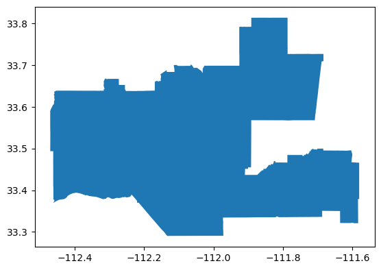

Date Summary: The 2020 TIGER/Line Arizona County Subdivisions dataset provides detailed administrative boundary information for the 61 county subdivisions in Arizona. It is available as a GeoDataFrame containing multiple attributes including geographic identifiers (GEOID), names, legal/statistical area descriptions, and precise boundary geometries. The dataset uses the NAD83 (EPSG:4269) coordinate system and is updated annually as part of the U.S. Census Bureau’s TIGER/Line program.

# Plot Phoenix area together with a base map

# Initialize figure
fig, ax = plt.subplots(figsize =(10, 10))

# Plot city boundary
phoenix.boundary.plot(ax=ax,
                     color='blue')
# Add base map
ctx.add_basemap(ax=ax, 
                # source=ctx.providers.CartoDB.Voyager, 
                crs=phoenix.crs)

# Clean map
ax.set_title('Map of Phoenix')
ax.axis('off')
ax.legend(phoenix['NAME'])

plt.show()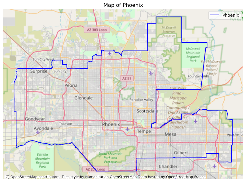

# Save file as GeoJSON for reproducibility
phoenix.to_file('data_clean/phoenix-boundary-file', driver='GeoJSON')

Now that we have Phoenix boundary mapped, we can move on to the Biodiversity Index dataset.

4. Access BII data from MPC

Workflow: - Define bounding box and time range for search - Open MPC catalog - Search MPC catalog for io_biodiversity collection with bounding box and time_range - Retrive search items - Select unique search item - Examine item.assets keys and title - Display pre-rendered image - Save data

# Define study extent and time range
bbox = [-112.826843, 32.974108, -111.184387, 33.863574]
time_range = "2017-01-01/2020-01-01"

# Access MPC catalog
catalog = Client.open(
    "https://planetarycomputer.microsoft.com/api/stac/v1",
    modifier=planetary_computer.sign_inplace,
)

# Search for collection 
search = catalog.search(
    collections=['io-biodiversity'],
    bbox=bbox,
    datetime=time_range)
search

# Retrieve items
items = search.item_collection()
items
# Determine number of items in search
print(f'There are {len(items)} items in the search.')

There are 4 items in the search.

item=items[0]
# Check assets in item 
for key in item.assets.keys():
    print(key, '--', item.assets[key].title)

data -- Biodiversity Intactness
tilejson -- TileJSON with default rendering
rendered_preview -- Rendered preview

# Plot rendered preview
Image(url=item.assets['rendered_preview'].href, width=500)

It seems that our biodiversity data is larger than phoenix. Let’s access the BII data and clip to study extent

Clip raster to geometry

# Explore data 
print(type(items))
print(len(items))
print(items[0].assets['data'].href)

<class 'pystac.item_collection.ItemCollection'>
4
https://pcdata01euw.blob.core.windows.net/impact/bii-v1/bii_2020/bii_2020_34.74464974521749_-115.38597824385106_cog.tif?st=2024-12-08T00%3A17%3A42Z&se=2024-12-09T01%3A02%3A42Z&sp=rl&sv=2024-05-04&sr=c&skoid=9c8ff44a-6a2c-4dfb-b298-1c9212f64d9a&sktid=72f988bf-86f1-41af-91ab-2d7cd011db47&skt=2024-12-08T03%3A52%3A20Z&ske=2024-12-15T03%3A52%3A20Z&sks=b&skv=2024-05-04&sig=aPPNFKqsw8IBhVdRMBurGkpa2RhJ7mc6qWmptB3E37s%3D

There’s only 1 dimension for band so it’s efficient to drop it using the squeeze() and .drop_vars()

# Select and process 2020 and 2017 data 
for idx in [0, 3]:
    # Load data
    bii = rioxr.open_rasterio(items[idx].assets['data'].href)
    # Drop band dimension 
    bii = bii.squeeze().drop_vars('band')
    
    # Match CRS and clip
    phoenix_match = phoenix.to_crs(bii.rio.crs)
    assert phoenix_match.crs == bii.rio.crs
    
    # Clip the raster to phoenix geometry
    year = '2020' if idx == 0 else '2017'
    globals()[f'bii_{year}_phoenix'] = (bii.rio.clip_box(*phoenix_match.total_bounds)
                                    .rio.clip(phoenix_match.geometry))

# Check clipped data
print(bii_2020_phoenix)
bii_2020_phoenix.plot()

<xarray.DataArray (y: 583, x: 990)> Size: 2MB
array([[nan, nan, nan, ..., nan, nan, nan],
       [nan, nan, nan, ..., nan, nan, nan],
       [nan, nan, nan, ..., nan, nan, nan],
       ...,
       [nan, nan, nan, ..., nan, nan, nan],
       [nan, nan, nan, ..., nan, nan, nan],
       [nan, nan, nan, ..., nan, nan, nan]], dtype=float32)
Coordinates:
  * x            (x) float64 8kB -112.5 -112.5 -112.5 ... -111.6 -111.6 -111.6
  * y            (y) float64 5kB 33.81 33.81 33.81 33.81 ... 33.29 33.29 33.29
    spatial_ref  int64 8B 0
Attributes:
    AREA_OR_POINT:  Area
    scale_factor:   1.0
    add_offset:     0.0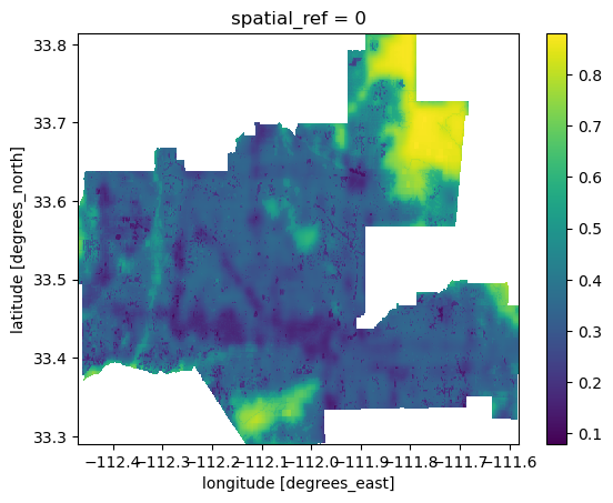

Calculate percent area with BII >0.75

To calculate percent area, we need total pixel counts of phoenix and then pixel counts with BII >= 0.75.

# Count total Phoenix pixels
total_counts = bii_2020_phoenix.count().item()
print(f"There are {total_counts} pixels in Phoenix")
# Select BII >= 0.75
over75_2020 = (bii_2020_phoenix >= 0.75).astype(int)
over75_2017 = (bii_2017_phoenix >= 0.75).astype(int)

There are 338699 pixels in Phoenix

# Count threshold pixels in 2020 
value, counts = np.unique(over75_2020, return_counts=True)
assert len(value) == len(counts)
# Initialize dictionary with column's data
dic = {'code': value,
       'counts': counts}
# Create a data frame 
pix_counts_20 = pd.DataFrame(dic)
pix_counts_20
# Report findings
print(f"There are {pix_counts_20.iloc[1,1]} pixels with BII >= 0.75 in 2020")

There are 21986 pixels with BII >= 0.75 in 2020

While it’s easy to run the same code for 2017, it’s better to write a for loop to maintain best coding practice.

# Count pixels with condition
years = {'2020': over75_2020, '2017': over75_2017}  # map years to their data

for year, data in years.items():
    # Count pixels for True/False
    value, counts = np.unique(data, return_counts=True)
    assert len(value) == len(counts)
    
    # Create dataframe
    dic = {'code': value, 'counts': counts}
    globals()[f'pix_counts_{year[-2:]}'] = pd.DataFrame(dic)  # creates pix_counts_20 and pix_counts_17
    
    # Save counts as variable

    globals()[f'counts_75_{year}'] = counts[1]
        
    # Report findings
    print(f"There are {counts[1]} pixels with BII >= 0.75 in {year}")

There are 21986 pixels with BII >= 0.75 in 2020
There are 24133 pixels with BII >= 0.75 in 2017

# Plot the data to check extent
over75_2017.plot()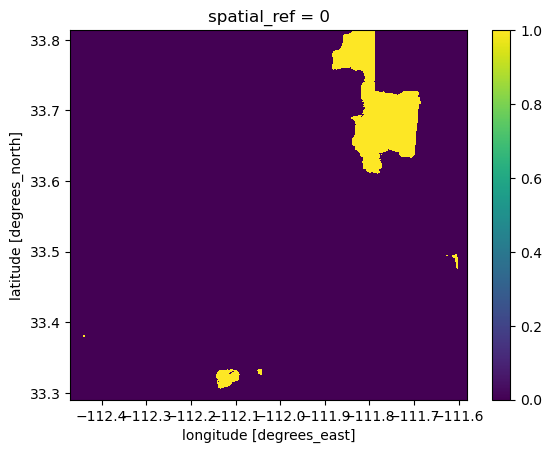

Now that we have pixel counts of both total cells in Phoenix and BII > 75% cells, we can calculate the percent area with a simple division.

# Write a "for loop" to run calculation for both years
ratio_2017 = round((counts_75_2017/total_counts)*100, 2)
ratio_2017

7.13

for year in years:
    # Calculate ratio
    globals()[f'ratio_{year}'] = (globals()[f'counts_75_{year}']/total_counts) * 100
    # Print result
    print(f"In {year}, {globals()[f'ratio_{year}']:.2f}% of pixels have BII >= 0.75")

In 2020, 6.49% of pixels have BII >= 0.75
In 2017, 7.13% of pixels have BII >= 0.75

# Obtain BII loss between 2017 to 2020
loss = over75_2017 - over75_2020
loss

<xarray.DataArray (y: 583, x: 990)> Size: 5MB
array([[0, 0, 0, ..., 0, 0, 0],
       [0, 0, 0, ..., 0, 0, 0],
       [0, 0, 0, ..., 0, 0, 0],
       ...,
       [0, 0, 0, ..., 0, 0, 0],
       [0, 0, 0, ..., 0, 0, 0],
       [0, 0, 0, ..., 0, 0, 0]])
Coordinates:
  * x            (x) float64 8kB -112.5 -112.5 -112.5 ... -111.6 -111.6 -111.6
  * y            (y) float64 5kB 33.81 33.81 33.81 33.81 ... 33.29 33.29 33.29
    spatial_ref  int64 8B 0

xarray.DataArray

• y: 583
• x: 990

• 0 0 0 0 0 0 0 0 0 0 0 0 0 0 0 0 0 ... 0 0 0 0 0 0 0 0 0 0 0 0 0 0 0 0

  array([[0, 0, 0, ..., 0, 0, 0],
         [0, 0, 0, ..., 0, 0, 0],
         [0, 0, 0, ..., 0, 0, 0],
         ...,
         [0, 0, 0, ..., 0, 0, 0],
         [0, 0, 0, ..., 0, 0, 0],
         [0, 0, 0, ..., 0, 0, 0]])

• Coordinates: (3)
  • x
    (x)
    float64
    -112.5 -112.5 ... -111.6 -111.6

    axis :

    X

    long_name :

    longitude

    standard_name :

    longitude

    units :

    degrees_east

    array([-112.469598, -112.468699, -112.467801, ..., -111.58296 , -111.582062,
           -111.581164])

  • y
    (y)
    float64
    33.81 33.81 33.81 ... 33.29 33.29

    axis :

    Y

    long_name :

    latitude

    standard_name :

    latitude

    units :

    degrees_north

    array([33.813546, 33.812648, 33.811749, ..., 33.292523, 33.291625, 33.290726])

  • spatial_ref
    ()
    int64
    0

    crs_wkt :

    GEOGCS["WGS 84",DATUM["WGS_1984",SPHEROID["WGS 84",6378137,298.257223563,AUTHORITY["EPSG","7030"]],AUTHORITY["EPSG","6326"]],PRIMEM["Greenwich",0,AUTHORITY["EPSG","8901"]],UNIT["degree",0.0174532925199433,AUTHORITY["EPSG","9122"]],AXIS["Latitude",NORTH],AXIS["Longitude",EAST],AUTHORITY["EPSG","4326"]]

    semi_major_axis :

    6378137.0

    semi_minor_axis :

    6356752.314245179

    inverse_flattening :

    298.257223563

    reference_ellipsoid_name :

    WGS 84

    longitude_of_prime_meridian :

    0.0

    prime_meridian_name :

    Greenwich

    geographic_crs_name :

    WGS 84

    horizontal_datum_name :

    World Geodetic System 1984

    grid_mapping_name :

    latitude_longitude

    spatial_ref :

    GEOGCS["WGS 84",DATUM["WGS_1984",SPHEROID["WGS 84",6378137,298.257223563,AUTHORITY["EPSG","7030"]],AUTHORITY["EPSG","6326"]],PRIMEM["Greenwich",0,AUTHORITY["EPSG","8901"]],UNIT["degree",0.0174532925199433,AUTHORITY["EPSG","9122"]],AXIS["Latitude",NORTH],AXIS["Longitude",EAST],AUTHORITY["EPSG","4326"]]

    GeoTransform :

    -112.47004683159909 0.0008983152841195194 0.0 33.81399511086966 0.0 -0.0008983152841195182

    array(0)

• Indexes: (2)
  • x
    PandasIndex

    PandasIndex(Index([-112.46959767395703, -112.46869935867291, -112.46780104338879,
           -112.46690272810467, -112.46600441282054, -112.46510609753642,
            -112.4642077822523, -112.46330946696818, -112.46241115168407,
           -112.46151283639995,
           ...
            -111.5892486955199, -111.58835038023577, -111.58745206495165,
           -111.58655374966753, -111.58565543438341,  -111.5847571190993,
           -111.58385880381518, -111.58296048853106, -111.58206217324694,
           -111.58116385796282],
          dtype='float64', name='x', length=990))

  • y
    PandasIndex

    PandasIndex(Index([  33.8135459532276, 33.812647637943485,  33.81174932265937,
            33.81085100737524,  33.80995269209112, 33.809054376807005,
            33.80815606152289,  33.80725774623877,  33.80635943095465,
           33.805461115670525,
           ...
           33.298811295427114, 33.297912980142996,  33.29701466485888,
            33.29611634957476,  33.29521803429064,  33.29431971900652,
             33.2934214037224,  33.29252308843828,  33.29162477315416,
            33.29072645787004],
          dtype='float64', name='y', length=583))

• Attributes: (0)

Value in loss variable represents change of BII between the years. 1 indicates BII loss, and -1 indicates BII gain, 0 means no change.

# Select xarray cells with value of 1 
loss = loss.where(loss==1)
loss
loss.plot()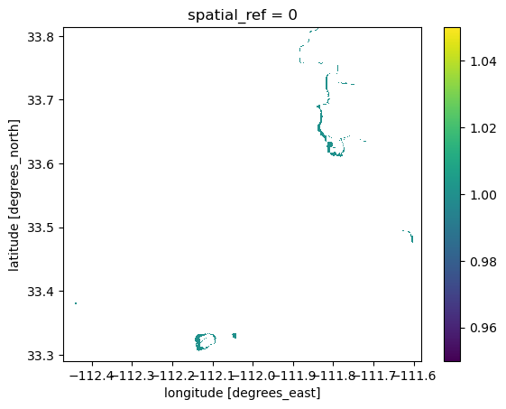

Visualize biodiversity loss

# Define aspect ratio with height and width
aspect = bii_2020_phoenix.rio.width/bii_2020_phoenix.rio.height

# Initialize figure
fig, ax = plt.subplots(figsize=(10, 4*aspect))

# Plot the BII raster in 2020
bii_2020_phoenix.plot(ax=ax,
                     cbar_kwargs={
                    "orientation": "horizontal",
                    "label": "BII for 2020"}
                     )

# Plot the loss layer
loss.plot(ax=ax,
         cmap="inferno",
         add_colorbar=False)

# Plot city boundary
phoenix.boundary.plot(ax=ax,
                     color='blue')

# Set legend for change raster
red_patch = mlines.Line2D([], [], color = "red", 
                          label = "Biodiversity area loss", 
                          linewidth = 4)

ax.legend(handles = [red_patch],
          bbox_to_anchor=(0, 0, 0.75, 0),
         fontsize = 8)

# Set title
ax.set_title("Biodiversity Intactness Index (BII) \nPhoenix Subdivision")

# Turn axis off
ax.axis("off")

plt.show()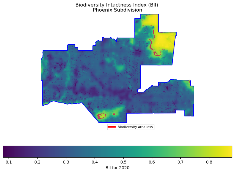

This figure shows the Biodiversity Intactness Index (BII) for the Phoenix Subdivision in 2020. The BII values are displayed using a color gradient scale ranging from 0.1 to 0.8. The area is outlined in blue, showing the subdivision boundaries. Quantitative analysis reveals a decline in high-biodiversity areas between 2017 and 2020. In 2017, 7.13% of the area had high biodiversity intactness (BII ≥ 0.75), which decreased to 6.49% by 2020. This decline is visually represented by the red areas marking “Biodiversity area loss,” which appear in two main locations: a larger area in the northeastern section of the subdivision and another smaller cluster in the southern portion.